A tuning fork density meter measures fluid density by vibrating a small fork-shaped element at its natural resonant frequency and reading how that frequency shifts when the fork is immersed in the process fluid. Because the resonant frequency of a vibrating element depends on the mass of the fluid it displaces, the frequency shift maps directly — through a calibrated curve — to density, and from density to concentration. This page explains the physics, the sensor construction, the measurement cycle, and the conditions where a tuning fork is the right choice.
What Is a Tuning Fork Density Meter
A tuning fork density meter is an inline or insertion instrument that determines the density (and, on dual-parameter models, the viscosity) of a liquid from the resonant behavior of a fork-shaped sensing element. The fork is typically manufactured from a single piece of stainless steel or Hastelloy, driven electromagnetically or piezo-electrically at its mechanical resonance, and kept vibrating continuously while the fluid flows past or around it.
Unlike a Coriolis mass flow meter, a tuning fork density meter does not require a flowing tube loop or full mass-flow measurement — it is a point-density sensor. Unlike a radiometric (nuclear) gauge, it contains no radioactive source. And unlike an ultrasonic meter, its sensing element is physically in contact with the fluid, which is precisely why it delivers higher accuracy on clean liquids but is vulnerable to coating and abrasion.
The Physics: Why Frequency Tells You Density
The fork behaves like a damped harmonic oscillator. Its natural resonant frequency ff is set by the stiffness kk of the fork and its effective vibrating mass meffmeff:
f=12πkmefff=2π1meffk
When the fork is immersed in a fluid, the fluid adds entrained (hydrodynamic) mass to the vibrating element. Denser fluid → more entrained mass → lower resonant frequency. The relationship is monotonic and, over the operating range of a given fork geometry, effectively linear. The instrument measures the resonant frequency with high resolution, then converts it to density using a factory calibration curve:
ρ=a⋅(f0−f)+bρ=a⋅(f0−f)+b
where f0f0 is the in-air or reference resonant frequency, and aa, bb are calibration constants determined during manufacturing against reference fluids (typically distilled water and a certified high-density standard).
Two physical effects are exploited at once on dual-parameter models:
-
- Resonant frequency shift → density
-
- Vibration amplitude damping (decrement) → viscosity
This is why a single tuning fork sensor can report both density and viscosity without a second element.
Inside the Sensor: Fork, Piezo, and Wetted Parts
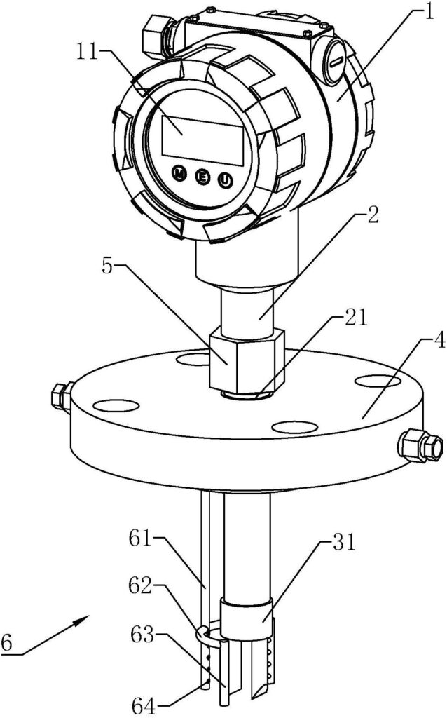
A typical inline tuning fork density transmitter contains:
-
- The fork element — two tines (or a single tuning-fork-shaped blade) machined from one billet. Geometry and material define the base frequency (commonly 400–2000 Hz depending on size and application).
-
- Drive/sense element — a piezo or electromagnetic coil that sustains oscillation and senses the actual resonant frequency. On a “self-exciting” design the circuit locks onto the fork’s natural frequency automatically.
-
- Wetted housing — the part exposed to process fluid, usually 316L stainless steel, Hastelloy, or a ceramic-coated variant for abrasive service. Process connection is flange, threaded, or hygienic tri-clamp.
-
- Electronics & transmitter — measures frequency, applies temperature compensation, computes density/concentration, and outputs the result.
For abrasive or erosive duty, the tines may be coated or made from technical ceramic (e.g. LONN-700C uses ceramic tines rated ~1200 HV), extending service life from weeks to months in slurry service.
The Measurement Cycle Step by Step
-
- Excitation — the drive circuit energizes the fork at its natural frequency and holds it in steady oscillation.
-
- Frequency sensing — the sense element reads the live resonant frequency, typically resolved to better than 0.01 Hz.
-
- Temperature read — an integral RTD (Pt100/Pt1000) measures fork temperature; the value feeds the compensation algorithm.
-
- Density conversion — firmware applies the calibration curve to convert frequency → density.
-
- Concentration conversion (optional) — if a density-to-concentration curve for the specific fluid is loaded, density is converted to % concentration at the reference temperature.
-
- Output — the computed value is sent as 4–20 mA, RS485/Modbus RTU, or HART to the DCS/PLC.
The cycle repeats continuously — there is no sampling, no laboratory step, and no process interruption.
Temperature Compensation Is Not Optional
Density and, more strongly, concentration are temperature-dependent. A 1 °C shift can move a concentration reading by a fraction of a percent — acceptable in some duties, unacceptable in custody transfer or tight blending. The tuning fork meter therefore measures fork temperature on every cycle and applies:
-
- Density temperature compensation using the fluid’s thermal expansion coefficient, and
-
- Concentration temperature compensation (TCM) using the fluid-specific density-vs-temperature-vs-concentration model loaded during configuration.
Proper TCM is what lets a tuning fork meter hold ±0.2% concentration accuracy across a 0–100% range on acids, bases, and solvents when temperature-compensated — a figure quoted for the LONN-700CM inline tuning fork meter.
From Density to Concentration
Many process plants do not care about absolute density; they care about concentration — % H₂SO₄, °Brix, % NaOH, % alcohol. Because density is a deterministic function of concentration at a fixed temperature for a given single-component-in-solvent system, the meter loads a pre-programmed density-to-concentration table (or a polynomial) and outputs concentration directly.
Caveat: density-to-concentration conversion is reliable for single dissolved species in a known solvent. It degrades when multiple species coexist or when the fluid composition is unknown — the meter cannot tell “which” solute is causing the density. State the fluid explicitly during configuration.
Typical Specifications You Can Expect
| Parameter | Typical tuning fork value | Note |
|---|---|---|
| Density range | 0–3 g/cm³ (model dependent) | Confirm against your fluid |
| Density accuracy | ±0.001 to ±0.002 g/cm³ | Clean, stable fluid |
| Density resolution | 0.0001 g/cm³ | High-resolution read |
| Repeatability | ±0.0002 to ±0.0005 g/cm³ | Short-term |
| Concentration accuracy | ±0.2% (TCM, single species) | Acids/bases/solvents |
| Response time | 1–5 s | Depends on damping |
| Process temperature | −25 to +150 °C (standard) | Higher on request |
| Output | 4–20 mA + RS485 Modbus (HART opt.) | Integrate to DCS/PLC |
| Wetted material | 316L / Hastelloy / ceramic | Match corrosion duty |
Published accuracy is only part of the story: installation quality, temperature compensation, and the specific fluid often matter more than the datasheet number. A well-installed meter can outperform a poorly installed one of a “better” class.
Installation: Inline, Insertion, and Wetted Materials
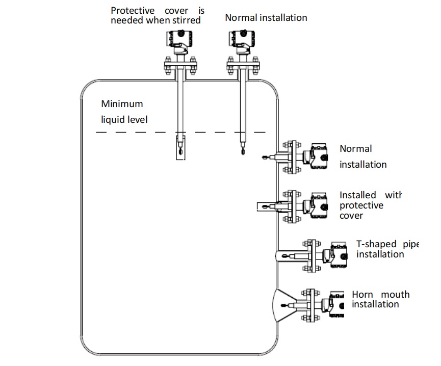
Tuning fork density meters are installed three ways:
-
- Inline (pipe tee / spool) — the fork sits in the flowing stream; best for representative, well-mixed process fluid.
-
- Insertion — the fork probes into a large pipe or tank through a nozzle; useful for retrofits.
-
- Sanitary / hygienic — tri-clamp or aseptic connection with drainable, smooth surfaces for 3-A / EHEDG duty.
Because the tines are immersed, installation must avoid:
-
- Air bubbles / vapor trapped on the fork (causes unstable reading),
-
- Dead legs and product retention (hygiene and cleaning),
-
- Severe vibration transmitted from the pipe (use supports/isolators).
Outputs and Integration
Standard outputs are 4–20 mA (density or concentration) plus RS485 Modbus RTU; HART is available on some models. The meter drops into a DCS, PLC, or SCADA without a separate analyzer rack, and supports alarm limits and datalogging at the controller. For custody transfer or tight concentration control, use the digital Modbus channel to carry the full-resolution value rather than the 4–20 mA span.
Where Tuning Fork Density Meters Excel
-
- Clean liquids and solutions — acids, bases, solvents, brines where the fork stays clean.
-
- Concentration control — sulfuric acid dilution (92–98% H₂SO₄), NaOH strength (10–50%), HCl pickling bath, solvent recovery (ethanol/methanol/IPA).
-
- Custody transfer of high-value fluids — high accuracy and no source licensing.
-
- Retrofit without shutdown — where a clamp-on ultrasonic cannot meet accuracy, an insertion tuning fork often can.
Honest Limitations
A tuning fork meter is not universal. Be straight about where it struggles:
-
- Abrasive slurry — particles erode the tines within weeks to months; ceramic tines (LONN-700C) help but ultrasonic remains superior here.
-
- Coating / fouling fluids — deposits on the fork shift the resonance and drift the reading until cleaned.
-
- Two-phase or aerated fluids — bubbles and solids destabilize the signal.
-
- Unknown multi-species fluids — density alone cannot resolve composition.
For slurry, hygienic non-intrusive, or “no wetted part” duties, compare with the ultrasonic principle. For a full technology map, see the technology comparison .
Tuning Fork vs Other Technologies
The tuned-fork principle is one of several inline density methods. The practical split:
-
- vs Ultrasonic — tuning fork wins on accuracy for clean fluids and adds viscosity; ultrasonic wins on slurry/sanitary/non-intrusive. Full breakdown: Tuning Fork vs Ultrasonic Density Meter.
-
- vs Coriolis — Coriolis adds mass flow but costs more and is bulkier; tuning fork is the lean point-density choice.
-
- vs Nuclear — tuning fork needs no source licensing, leak testing, or decommissioning. See the non-nuclear discussion.
Recommended LONNMETER Instruments
| Model | Principle | Best for | Key spec |
|---|---|---|---|
| LONN-700CM | Inline tuning fork | Clean liquids, custody transfer, acid/base concentration | ±0.002 g/cm³; 4–20 mA + Modbus |
| LONN-700C | Ceramic tuning fork | Abrasive slurry (small particles) | Ceramic tines ~1200 HV; ±0.002 g/cm³ |
| LONN-V7 | Tuning fork (dual) | Density + viscosity (coatings, adhesives, polymers) | Dual-parameter, single sensor |
Browse the full range: LONNMETER inline density meter product range · See all density technologies in the Density Measurement Hub.
Frequently Asked Questions
Q1: How does a tuning fork density meter actually measure density?
It vibrates a fork-shaped element at its natural resonant frequency. The surrounding fluid adds mass to the vibrating element, lowering the frequency. The instrument measures that frequency shift and converts it to density through a factory calibration curve.
Q2: Why is temperature compensation necessary?
Density and concentration are temperature-dependent; a 1 °C change can shift a concentration reading by a fraction of a percent. The meter reads fork temperature every cycle and applies fluid-specific compensation so the output stays accurate across the process temperature range.
Q3: How accurate is a tuning fork density meter?
Typical density accuracy is ±0.001 to ±0.002 g/cm³ on clean, stable fluids, with ±0.2% concentration accuracy (temperature-compensated) for single-species acids, bases, and solvents. Real-world accuracy also depends on installation and fluid condition.
Q4: What fluids should a tuning fork density meter NOT be used for?
Avoid abrasive slurries (erode the tines), heavy coating/fouling fluids (drift the reading), aerated or two-phase fluids (destabilize the signal), and unknown multi-species mixtures (density cannot resolve composition). For slurry, prefer ultrasonic.
Q5: Tuning fork vs ultrasonic — which do I choose?
Match to the fluid. Tuning fork for clean liquids, high accuracy, and density+viscosity; ultrasonic for slurry, hygienic non-intrusive service, and no wetted element. See the full comparison: Tuning Fork vs Ultrasonic Density Meter.
Q6: Does it need a radioactive source like nuclear density meters?
No. Tuning fork meters are non-radioactive. That removes source licensing, periodic leak testing, and decommissioning procedures required for radiometric gauges — a meaningful compliance and safety advantage.
Q7: How fast does it respond?
Response time is typically 1–5 seconds depending on fluid damping, with continuous output — no sampling or laboratory step.
Discuss your application: contact the LONNMETER technical team for a measurement review of your specific fluid, concentration range, and accuracy requirement.