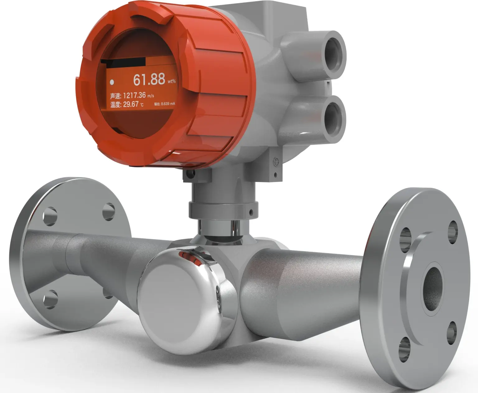
An ultrasonic density meter measures the density (and, for many liquids, the concentration) of a fluid without a vibrating or moving element. Instead of weighing a sample or tracking a resonating fork, it sends a high-frequency sound pulse through the liquid and measures how fast that pulse travels. Because the speed of sound in a liquid is tied to its density and composition, the transit time of the pulse becomes a direct window into what is flowing.

This guide explains the physics, the sensor construction, the measurement cycle, and the practical limits — so you can judge whether ultrasonic is the right principle for your duty, and how it differs from a tuning fork or Coriolis meter.
dn25 h.17

What Is an Ultrasonic Density Meter

An ultrasonic density meter is an inline or clamp-on instrument that determines fluid density from the velocity of sound in the process liquid. A pair of piezoelectric transducers (or one transducer plus a reflector) launches an acoustic pulse across a known path length inside the spool piece. The electronics time the flight of that pulse to picosecond resolution, convert the transit time into a sound speed, and then apply a fluid-specific calibration to report density — or, for a known binary mixture, concentration.The defining feature is the absence of any oscillating mechanical part in the measurement zone. There is no fork to foul, no U-tube to stress, and (in the clamp-on variant) no wetted surface at all. That is what makes ultrasonic attractive for abrasive slurries, hygienic duty, and retrofit without shutdown.

The Physics: Sound Speed Tells You Density

Sound travels through a liquid at a speed set by the fluid's bulk modulus K and its density ρ:

c = √(K / ρ)

where c is the speed of sound. For a given fluid at fixed temperature and pressure, K is effectively constant, so a change in c reflects a change in ρ. Measure c precisely and you can back out density.

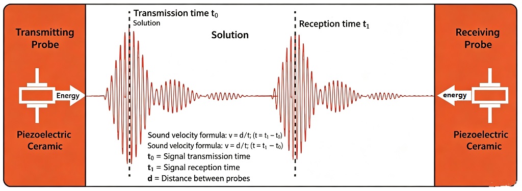
In practice the meter does not solve that equation live — it measures the one-way transit time Δt across a fixed acoustic path L:

c = L / Δt

If the instrument measures a round trip, Δt is half the measured time. The path length L is a manufactured constant; the only unknown the meter must resolve is the time of flight, which modern electronics resolve to better than a nanosecond.

The honest caveat: K is not a universal constant. It shifts with temperature, pressure, and — critically — fluid composition. Two liquids with the same density can have different sound speeds, and the same liquid at two concentrations has two sound speeds. That is why an ultrasonic meter reports density through a calibration, not from the physics equation alone (see "From Sound Speed to Density and Concentration").
figures vary by model and fluid

Sensor Construction: Transducers, Wafer, and Electronics

A typical inline ultrasonic density transmitter has three parts:

  • Acoustic cell (spool piece / wafer): a short section of pipe with two piezo-ceramic transducers mounted opposite each other, or one transducer facing a polished reflector. The bore is sized to the line; wetted materials are usually 316L stainless steel, with Hastelloy or ceramic options for corrosive or abrasive service.
  • Transducers: piezoelectric elements that convert electrical pulses into sound and back. They are tuned to a few MHz. In the clamp-on variant the transducers sit on the outside of the existing pipe and couple through the wall — no process contact.
  • Electronics housing: a transmitter that generates the pulse, times the return, reads a Pt100 temperature element, runs the calibration and compensation math, and drives the output. It is typically rated IP65/IP67 and mounted locally or remotely.

The clamp-on version deserves a call-out: because the sound must cross the pipe wall before reaching the liquid, its accuracy depends on wall thickness, material, and coupling. It trades some precision for true non-intrusive installation — ideal for retrofits and lines that cannot be opened.

The Measurement Cycle Step by Step

  1. The transmitter fires an ultrasonic pulse from the send transducer.
  2. The receive transducer (or reflector path) captures the pulse; the time interval counter records the flight time Δt.
  3. The firmware computes sound speed c = L / Δt.
  4. A temperature element reads process temperature T.
  5. A fluid-specific calibration model converts (c, T) into density ρ — or, for a binary mixture, into concentration.
  6. The result is filtered and pushed to the output (4-20 mA, Modbus, HART) and to any local display.

The cycle repeats several times per second, so the instrument tracks density and concentration in near-real time rather than as a slow lab sample.

From Sound Speed to Density and Concentration

This is the step beginners miss. The meter measures sound speed directly; density is derived. For a single-component liquid at known T and P, a calibration maps c → ρ. For a two-component mixture (say acid-in-water, or sugar-in-water), both density and sound speed vary with the blend ratio, so measuring c together with T yields concentration directly — Brix, % mass, °Bé, or whatever the mixture's calibration expresses.

Calibration is usually a polynomial or look-up table supplied for the specific fluid:


ρ = f(c, T) (fluid-specific, established by factory or field calibration)

The practical implication: an ultrasonic density meter is only as good as its calibration for your fluid. A generic sound-speed reading is not a density reading until the calibration for that liquid is loaded. This is the main difference from a tuning fork, which infers density more directly from a resonant frequency shift.

Temperature Compensation and Why It Matters

Sound speed is strongly temperature-dependent — for water it falls by roughly 2.5 m/s per °C. Uncompensated, a few degrees of temperature drift would swamp the density signal. That is why every ultrasonic density cell carries a temperature element and the calibration is a function of (c, T), not c alone.When specifying the instrument, confirm the calibration covers your full operating temperature band. A meter calibrated at 20 °C will read off-target at 80 °C unless the T term is in the model.

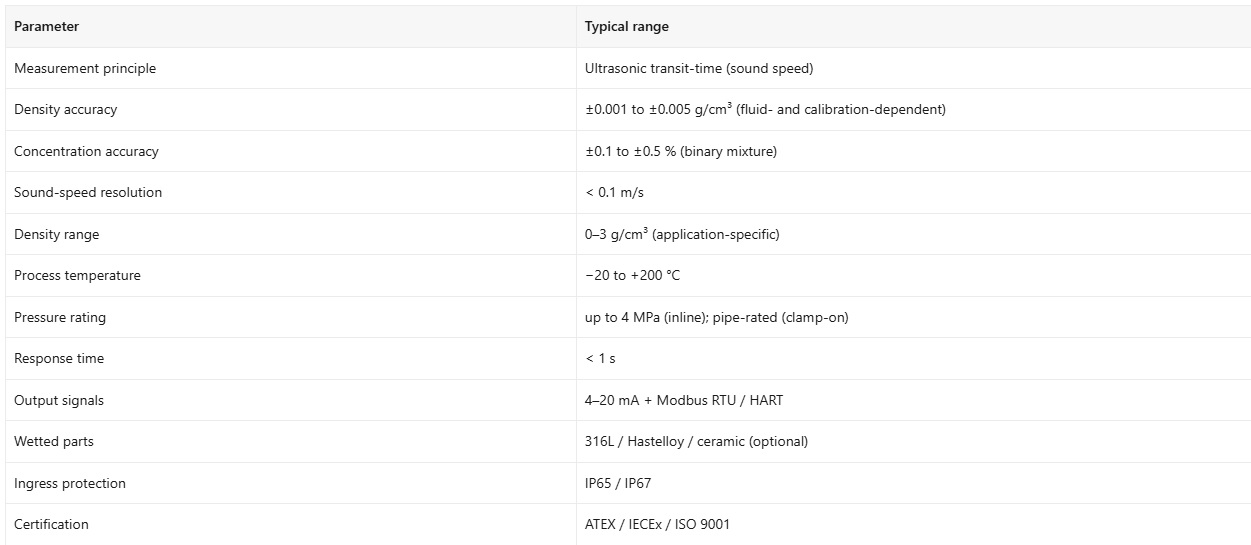
Typical Specifications

Values below are typical for industrial inline ultrasonic density/concentration transmitters. Confirm against the actual datasheet before quoting to a customer — figures vary by model and fluid.
figures vary by model and fluid

Outputs, Installation, and Integration

Ultrasonic density meters speak the same control-room language as other inline instruments: a 4–20 mA loop for density or concentration, plus a digital bus (Modbus RS-485 or HART) for diagnostics, temperature, and secondary variables. They drop into a DCS or PLC like any other transmitter and need no radioactive source permit — unlike radiometric gauges.
Inline wafer cells install in a straight run with appropriate upstream/downstream piping; clamp-on units strap onto the existing line. Both avoid the special licensing, periodic source-leak testing, and decommissioning burden of nuclear density measurement.

Ultrasonic vs Tuning Fork: A Brief Comparison

Both are non-radioactive inline technologies, but they sense density differently:

  • Tuning fork measures the resonant frequency of a vibrating element immersed in the fluid; density shifts that frequency. It is direct and robust for clean-to-moderate liquids.
  • Ultrasonic measures sound speed across a path and derives density by calibration. It has no wetted vibrating part and handles higher solids loadings and non-intrusive (clamp-on) mounting better.

For the full side-by-side — accuracy, slurry limits, hygienic options, and which LONNMETER model fits which duty — see our dedicated comparison: Tuning Fork vs Ultrasonic Density Meter. The deeper technology round-up is in the Inline Density Measurement Methods Guide.

Where Ultrasonic Excels — and Where It Doesn't

Strengths

  • No moving or vibrating part in the measurement zone — less prone to mechanical fatigue.
  • Clamp-on option enables retrofit without cutting the line or stopping the process.
  • Tolerates high solids loadings (mining slurries up to ~40 % solids / 5 mm particles with the right model).
  • Fast, continuous reading suitable for closed-loop control.

Limitations

  • Gas bubbles and heavy suspended solids scatter or absorb the acoustic pulse, weakening the signal; de-gassing or an alternative principle may be needed.
  • Requires a fluid-specific calibration; a generic install will not read density correctly.
  • Temperature drift must be compensated or accuracy collapses.
  • Clamp-on accuracy is lower and sensitive to pipe-wall condition.
  • Stratified or off-path flow can give a non-representative reading if the acoustic path misses the bulk fluid.

Recommended LONNMETER Models

Model

Principle / mount

Best fit

Key spec

LONN7000

Inline ultrasonic

Mining slurry (up to 40 % solids, 5 mm particles); sanitary 3-A / CIP version for food, dairy, pharma

Non-radioactive, ATEX/IECEx/ISO 9001

LONN-UFM

Clamp-on ultrasonic

Retrofit without shutdown; lines that cannot be opened

Non-intrusive installation

LONN7001

Tee ultrasonic density/concentration

Online density + concentration from one tee

See product overview

All LONNMETER models use non-radioactive measurement, carry ATEX / IECEx / ISO 9001 certification, and are supported across 130+ countries. For model availability and the exact detail page, confirm with LONNMETER .

Need help choosing between ultrasonic, tuning fork, or Coriolis for your specific fluid? Our density meter selection guide walks the decision, or talk to an application engineer via contact.

Frequently Asked Questions

Q1: How does an ultrasonic density meter actually measure density?

It times an ultrasonic pulse across a known path through the liquid, converts the transit time into a sound speed, then applies a fluid-specific calibration (sound speed + temperature → density). It does not weigh a sample; it infers density from how fast sound travels.

Q2: Is ultrasonic more accurate than tuning fork? 

Not inherently. Tuning fork reads density more directly from a resonant frequency; ultrasonic needs a calibration but handles higher solids and non-intrusive mounting. Accuracy depends on fluid, calibration quality, and install — see the comparison guide.

Q3: Can it handle slurries and suspended solids?

Yes, within limits — inline ultrasonic models handle mining slurries up to roughly 40 % solids and 5 mm particles. The bigger enemy is gas bubbles, which scatter the acoustic pulse.

Q4: What happens if there are gas bubbles in the line?

Bubbles weaken or kill the acoustic signal and bias the reading. De-gas the stream, place the meter on a bubble-free run, or consider a different principle (e.g., tuning fork or Coriolis) for gassy duty.

Q5: Clamp-on vs inline — which is more accurate?

Inline wafer cells are more accurate and repeatable. Clamp-on trades precision for true non-intrusive install; its reading depends on pipe-wall thickness, material, and coupling quality.

Q6: Does it need calibration?

Yes. Ultrasonic measures sound speed; density comes from a fluid-specific calibration. Factory calibration covers the specified fluid; field re-calibration may be needed if the process fluid changes.

Q7: How does temperature affect the measurement?

Sound speed drops with temperature (≈2.5 m/s per °C for water). The meter reads temperature and compensates in the calibration model — but the calibration must cover your operating temperature band.

Q8: Can it measure concentration, not just density?

For a known binary mixture, yes. Because both density and sound speed vary with blend ratio, measuring sound speed plus temperature yields concentration (Brix, % mass, etc.) directly via calibration.

Leave a Reply

Your email address will not be published. Required fields are marked *